43 conditional formatting data labels excel
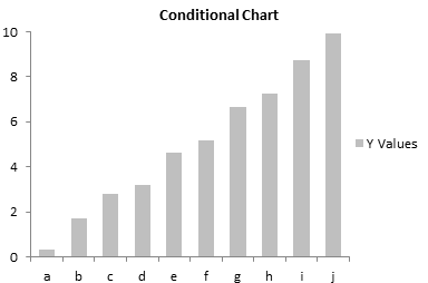
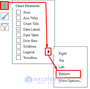
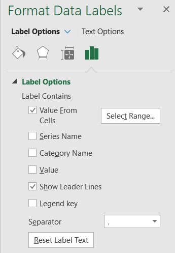
Change the format of data labels in a chart To get there, after adding your data labels, select the data label to format, and then click Chart Elements > Data Labels > More Options. To go to the appropriate area, click one of the four icons ( Fill & Line, Effects, Size & Properties ( Layout & Properties in Outlook or Word), or Label Options) shown here. How to Create Excel Charts (Column or Bar) with Conditional Formatting ... Conditional formatting is the practice of assigning custom formatting to Excel cells—color, font, etc.—based on the specified criteria (conditions). The feature helps in analyzing data, finding statistically significant values, and identifying patterns within a given dataset.
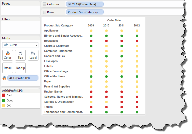
Conditional Formatting Using Custom Measure - Power BI Sep 28, 2020 · Voila! We have given conditional formatting to Day of Week column based on the clothing Category value. I just tried to add a simple legend on the top to represent the color coding. So, this is how one can use a custom color formatting in Power BI by creating a simple measure for it. Hope this article helps everyone out there. - Pragati
Conditional formatting data labels excel
How to change chart axis labels' font color and size in Excel? Sometimes, you may want to change labels' font color by positive/negative/ in an axis in chart. You can get it done with conditional formatting easily as follows: 1. Right click the axis you will change labels by positive/negative/0, and select the Format Axis from right-clicking menu. 2. A Comprehensive guide to Microsoft Excel for Data Analysis Nov 24, 2021 · The following approaches can be used to clean data in Excel. • With Text Functions • Containing Date Values • Containing Time Values. 3) Conditional Formatting. Conditional formatting instructions in Excel allow you to colour cells or fonts, as well as place symbols next to values in cells, based on predetermined criteria. Conditional formatting Data Bars in Excel - ablebits.com To insert data bars in Excel, carry out these steps: Select the range of cells. On the Home tab, in the Styles group, click Conditional Formatting. Point to Data Bars and choose the style you want - Gradient Fill or Solid Fill. Once you do this, colored bars will immediately appear inside the selected cells.
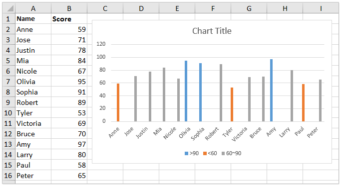
Conditional formatting data labels excel. Microsoft Excel conditional number formatting Sep 17, 2019 · Next, I would apply conditional formatting number formatting where the cell value is greater than one so that numbers greater than a million could be displayed to the nearest 0.1m, numbers less than a million but greater than or equal to 1,000 could be displayed to the nearest 0.00k and numbers lower than 1,000 (but necessarily greater than one ... How to create a chart with conditional formatting in Excel? - ExtendOffice Select the chart you want to add conditional formatting for, and click Kutools > Charts > Color Chart by Value to enable this feature. 2. In the Fill chart color based on dialog, please do as follows: (1) Select a range criteria from the Data drop-down list; (2) Specify the range values in the Min Value or Max Value boxes; (3) Choose a fill ... Excel Data Analysis - Conditional Formatting - tutorialspoint.com Click the blue data bar in the Gradient Fill options. Repeat the first three steps. Click the blue data bar in the Solid Fill options. You can also format data bars such that the data bar starts in the middle of the cell, and stretches to the left for negative values and stretches to the right for positive values. Use conditional formatting to highlight information Conditional formatting can help make patterns and trends in your data more apparent. To use it, you create rules that determine the format of cells based on their values, such as the following monthly temperature data with cell colors tied to cell values.
r/excel - Is it possible to conditionally format Data Labels on a ... On a dynamic line chart, where Y-axis is scaled from 0-10 and X-axis is dates, is it possible to conditionally format Data Labels such that the colour of the data labels changes based on the data values that are plotted. For example, when numbers 0-3 are plotted on the dynamic chart above their data label's font colour turns red, and if numbers ... How to Apply Conditional Formatting to Pivot Tables - Excel … Dec 13, 2018 · How to Setup Conditional Formatting for Pivot Tables. Setting up conditional formatting for pivot tables is a little different than it is for regular cells/ranges. So in this post I explain how to apply conditional formatting for pivot tables. 1. Select a cell in the Values area. The first step is to select a cell in the Values area of the ... How to Use Microsoft Excel: Complete Beginner's Guide 40+ Tips - wikiHow Sep 19, 2022 · To instantly apply conditional formatting (which is usually a little more complex in Excel) based on your data, use the Formatting tab. ... line, or bar, you'll see options you can edit in the panel on the right side of excel. Here you can change the axis labels, alignment, and legend data. Advertisement. Community Q&A Search. Add New Question. Can I use conditional formatting to change colors depending on data values? To set up conditional formatting, select the respective data cells in the Excel file. For line charts, the fill color of data cells controls the color of markers (see Line scheme). The line color itself is controlled by the cell containing the line series label. These cells may contain any number format, formulas, and references to other cells.
Invert if Negative Formatting in Excel Charts - Peltier Tech Dec 05, 2019 · This might be fine in a line chart, to move the axis labels out of the way of the data. In a bar or column chart, this isn’t a good idea. Since Excel draws bars and columns starting from the axis, you get excessively long positive bars for positive values, and short positive bars for negative values. Top Microsoft Excel Training Course (2021 Update) How to Customize Chart Titles and Legends in Excel . Gridlines, Labels, and Data Tables How to Display Chart Gridlines, Labels, and Data Tables in Excel . Chart Elements How to Format Chart Data in Excel . Modify Chart Data How to Modify Chart Data in Excel . Trendlines How to Add Trendlines in Excel . Dual-Axis Charts Excel conditional formatting formulas based on another cell - Ablebits.com On the Home tab, in the Styles group, click Conditional formatting > New Rule…; In the New Formatting Rule window, select Use a formula to determine which cells to format.; Enter the formula in the corresponding box. Click the Format… button to choose your custom format.; Switch between the Font, Border and Fill tabs and play with different options such as font style, pattern color and ... Paste TO visible cells only in a filtered cells only Nov 17, 2019 · Labels: Labels: Excel; Formulas and Functions ... It is a shame that there isn't a way to inform Excel that the pasted data should only be deposited into visible cells. Have a good one. 1 Like . Reply. ... you can always use conditional formatting to identify and highlight any matching cells in a column from one sheet to another within the same ...
Conditional Formatting of Excel Charts - Peltier Tech
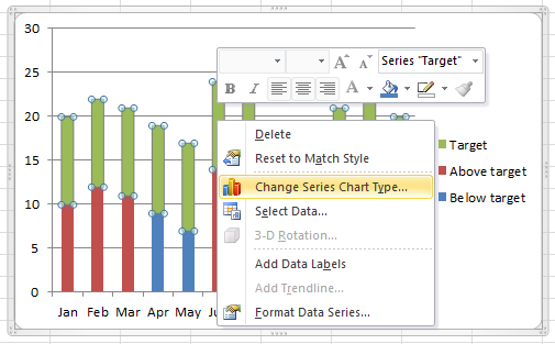
Conditional formatting chart data labels? - Excel Help Forum The easy way to conditionally format these labels is use two series. Use something like =IF ($E2=1,0,NA ()) for the series that has red labels and =IF (#E2=1,NA (),0) for the series that has unformatted labels. Jon Peltier Register To Reply Similar Threads Conditional Number Formatting Not Working for Chart Value Labels

Dynamically Label Excel Chart Series Lines • My Online ...
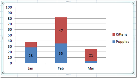
Conditional formatting on Pivot Chart - Microsoft Community Answer. not with a pivot chart, unless you change the underlying table. Conceptually, "conditional formatting of columns" is not a feature of charts. The workaround is to create a data series for each "color" and use these different series instead of the original single data series in a stacked column chart. Only one series in each stack has a ...

Conditional Formatting
Conditional Formatting in Excel - a Beginner's Guide - GoSkills.com Excel has a tool that automatically helps you out with that — it's called conditional formatting. If you're ready to take your data organization game to the next level, keep reading to learn how to use conditional formatting in Excel. In this resource, we'll apply conditional formatting to a pivot table. Note that the steps to apply pivot ...

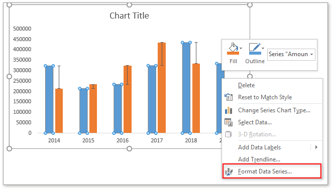
Change the format of data labels in a chart
Conditional Formatting in Excel - Step by Step Examples - WallStreetMojo The conditional formatting excel feature changes the appearance of a cell by changing its fill color, border, font color, and so on. With such changes, certain data cells can be distinguished from the others. This feature is available in the "styles" group of the Home tab. A conditional formatting rule in excel can fulfill a variety of conditions.

Solved: Bar Chart Data Labels - Conditional Formatting - W ...
Creating Conditional Data Labels in Excel Charts - YouTube We can make labels appear on our charts that don't have to do with the raw numbers that built the chart - and we can make them show up or not based on whatever conditions we want. In this tutorial,...
Conditional Formatting
Conditional Label Formatting in Excel Charts : r/excel The user can edit the metric they look at using a drop down list (created with conditional formatting). The data is then displayed in both a table and a chart. The table compromises of just two columns; one with the product name and one with the metric that the user has chosen e.g. £ value sales or % sold on promotion.
Excel Bar Graph Color with Conditional Formatting (3 Suitable ...
Conditional formatting for chart axes - Microsoft Excel 365 Apply standard conditional formatting for axes. To change the format of the label on the Excel for Microsoft 365 chart axis (horizontal or vertical, depending on the chart type), do the following: 1. Right-click on the axis and choose Format Axis... in the popup menu: 2.

Enable or Disable Excel Data Labels at the click of a button ...
Conditional format chart data labels | Dashboards & Charts | Excel Forum Lance 354 524 550. I create a bar chart that from this data, and display the data label for Actual. I would like to format this data label so that it displays in Red if the value of Actual is less than the value of On Track. Otherwise, it will just display as Blue, which is the format color right now. I tried Conditional Formatting on the data ...
Power BI Dynamic Conditional Formatting
Time Series Data Models in SQL Server and Excel to Visualize Data Visually Modeling SQL Server Data in Excel with Conditional Formatting and Line Charts. ... Columns A, B, C, and G in the first worksheet row show column labels for the symbol, date, ema_10, and open column values from the SQL Server table. Columns D, E, F, and H are hidden columns with contents for other columns from the denormalized_emas_by ...
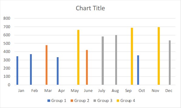
Conditional formatting for Excel column charts | Think ...
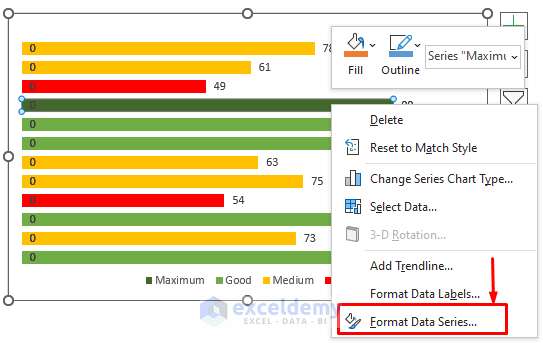
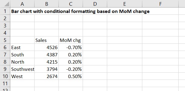
Excel bar chart with conditional formatting based on MoM change Click on any bar and press Ctrl+1 to make the Format Data Series task pane appear if it is not already showing. In the Series Options section, set the Gap Width to 50% to give the bars more presence and set the Series Overlap to 100%. Use the chart skittle (the "+" sign to the right of the chart) to remove the legend and gridlines.

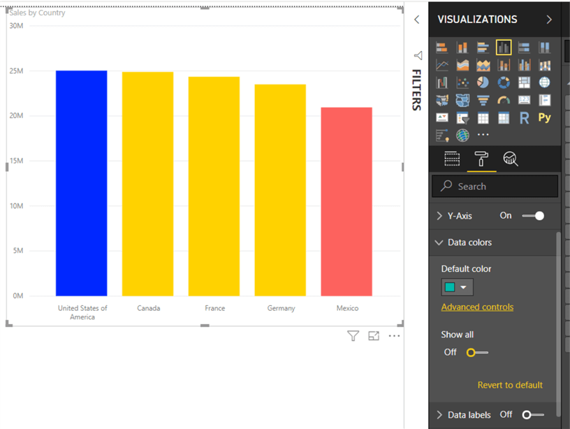
Conditional formatting by field value in Power BI - Power BI Docs
Conditional format of chart labels - Excel Help Forum Whilst Conditional Formatting will not be pickup by the data labels there may be alternative approaches before reverting to VBA. Custom number format could control colour. Additional series in the chart could provide differently formatted labels. Can you post example and detail of what the CF is. Cheers Andy Register To Reply
How to create a chart with conditional formatting in Excel?
Conditional formatting for Data Labels in Power BI Where you can find the conditional formatting options? Select the visual > Go to the formatting pane> under Data labels > Values > Color Data Labels Let's Get Started- Add one line chart visual into page and create two measure for Profit & Sales. Note: If you don't want to create measure then you can directly use Sales and Profit fields.
Excel Bar Graph Color with Conditional Formatting (3 Suitable ...
10 spiffy new ways to show data with Excel | Computerworld Select a range of data, click the Conditional Formatting item in the Ribbon, and click Icon Sets, then one of the simple options under Directional. Now each data cell displays an arrow icon.

Color Negative Chart Data Labels in Red with downward arrow
How-to Make Conditional Data Labels for an Excel Dashboard Checkout the Step-by-Step Tutorial here: on How to conditionally hide and unhide data labels ...
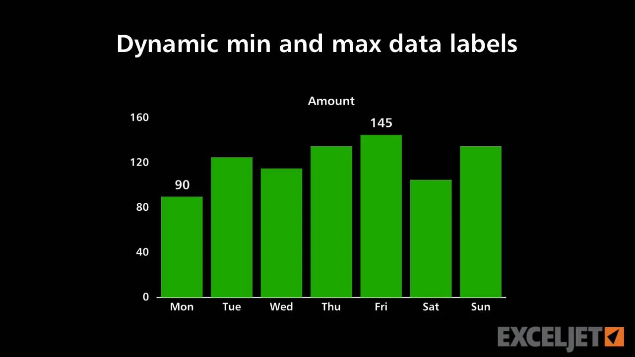
Dynamic min and max data labels
Data Tables & Monte Carlo Simulations in Excel - Chandoo.org May 06, 2010 · The Data Table function is a function that allows a table of what if questions to be posed and answered simply, and is useful in simple what if questions, sensitivity analysis, variance analysis and even Monte Carlo (Stochastic) analysis of real life model within Excel. The Data Table function should not be confused with the Insert Table function.
Step by step to create a column chart with percentage change ...
Conditional formatting Data Bars in Excel - ablebits.com To insert data bars in Excel, carry out these steps: Select the range of cells. On the Home tab, in the Styles group, click Conditional Formatting. Point to Data Bars and choose the style you want - Gradient Fill or Solid Fill. Once you do this, colored bars will immediately appear inside the selected cells.

How to insert data labels to a Pie chart in Excel 2013
A Comprehensive guide to Microsoft Excel for Data Analysis Nov 24, 2021 · The following approaches can be used to clean data in Excel. • With Text Functions • Containing Date Values • Containing Time Values. 3) Conditional Formatting. Conditional formatting instructions in Excel allow you to colour cells or fonts, as well as place symbols next to values in cells, based on predetermined criteria.
Excel bar chart with conditional formatting based on MoM ...
How to change chart axis labels' font color and size in Excel? Sometimes, you may want to change labels' font color by positive/negative/ in an axis in chart. You can get it done with conditional formatting easily as follows: 1. Right click the axis you will change labels by positive/negative/0, and select the Format Axis from right-clicking menu. 2.

Enhance the Card Visual in Power BI with Conditional ...
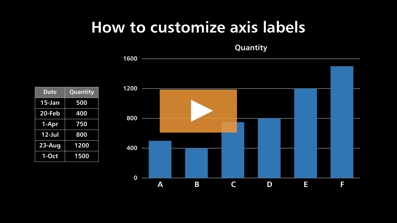
How to customize axis labels
Example: Charts with Data Labels — XlsxWriter Documentation

Custom Data Labels with Colors and Symbols in Excel Charts ...

Custom data labels in a chart

Is it possible to conditionally format Data Labels on a ...
Excel bar chart with conditional formatting based on MoM ...

Apply Custom Data Labels to Charted Points - Peltier Tech

Custom Excel Chart Label Positions • My Online Training Hub

Apply Custom Conditional Formatting to Clustered Column Chart ...
How-to Make Conditional Label Values in an Excel Stacked ...
/Capture-e92aa05671d543ceaf94080eb2687619.JPG)
Understanding Excel Chart Data Series, Data Points, and Data ...

Color Negative Chart Data Labels in Red with downward arrow

Custom Data Labels with Colors and Symbols in Excel Charts ...

Conditional Formatting of Data Labels on Chart - Microsoft ...
How to improve or conditionally format data labels in Power ...
Create charts with conditional formatting – User Friendly

How to improve or conditionally format data labels in Power ...
Google Workspace Updates: New chart text and number ...

Creating Conditional Data Labels in Excel Charts | Everyday Office 075

Change the format of data labels in a chart
How to change chart axis labels' font color and size in Excel?
How to add and customize chart data labels

Module1

Dynamic Number Format for Millions and Thousands - PK: An ...
Post a Comment for "43 conditional formatting data labels excel"