43 axis labels excel 2013

How to Add Leader Lines in Excel? - GeeksforGeeks Step 2: Go to Insert Tab and select Recommended Charts. A dialogue box name Insert Chart appears. Step 3: Click on All Charts and select Line. Click Ok. Step 4: A line chart is embedded in the worksheet. Step 5: Go to Chart Design Tab and select Add Chart Element . Step 6: Hover on the Data Labels option. Click on More Data Label Options …. Pivot chart X axis labels not aligned to the ... - Excel Help Forum I may not be the best one to walk you through the steps, since my older version of Excel might use a different interface. Basically: 1) Select either data series (I selected one of the orange bars).

Use defined names to automatically update a chart range - Office On the Insert tab, click a chart, and then click a chart type. Click the Design tab, click the Select Data in the Data group. Under Legend Entries (Series), click Edit. In the Series values box, type =Sheet1!Sales, and then click OK. Under Horizontal (Category) Axis Labels, click Edit.

Axis labels excel 2013

How to Make an Excel Box Plot Chart - Contextures Excel Tips To create the Box Plot chart: Select cells E3:G3 -- the heading cells -- then press Ctrl and select E10:G12. On the Excel Ribbon, click the Insert tab, and click Column Chart, then click Stacked Column. If necessary, click the Switch Row/Column command on the Ribbon's Design tab, to get the box series stacked. Click on the Base series to select ... Formatting axis labels on a paginated report chart - Microsoft Report ... Right-click the axis you want to format and click Axis Properties to change values for the axis text, numeric and date formats, major and minor tick marks, auto-fitting for labels, and the thickness, color, and style of the axis line. To change values for the axis title, right-click the axis title, and click Axis Title Properties. Format Chart Axis in Excel - Axis Options However, In this blog, we will be working with Axis options, Tick marks, Labels, Number > Axis options> Axis options> Format Axis Pane. Axis Options: Axis Options There are multiple options So we will perform one by one. Changing Maximum and Minimum Bounds The first option is to adjust the maximum and minimum bounds for the axis.

Axis labels excel 2013. Reading Values from Graphs (Microsoft Excel) Choose the Add Trendline option from the Context menu. Excel displays the Format Trendline dialog box. (See Figure 2.) Figure 2. The Format Trendline dialog box. Make sure the regression type you want to use is selected. Make sure the Display Equation on Chart check box is selected. Click on OK. Excel Bubble Chart Timeline Template - Vertex42.com STEP 6: ADD EVENT LABELS. Right-click on the event series and select Add Data Labels. Right-click again on the event series and select Format Data Labels. Like before with the axis, choose Value From Cells then select the range of labels from your table. Choose Above for the Label Position, and uncheck the Y Value. How to Create and Customize a Treemap Chart in Microsoft Excel Simply click that text box and enter a new name. Next, you can select a style, color scheme, or different layout for the treemap. Select the chart and go to the Chart Design tab that displays. Use the variety of tools in the ribbon to customize your treemap. For fill and line styles and colors, effects like shadow and 3-D, or exact size and ... How to Print Labels from Excel - Lifewire To label chart axes in Excel, select a blank area of the chart, then select the Plus ( +) in the upper-right. Check the Axis title box, select the right arrow beside it, then choose an axis to label. How do I label a legend in Excel? To label legends in Excel, select a blank area of the chart.

Date Axis in Excel Chart is wrong • AuditExcel.co.za In order to do this you just need to force the horizontal axis to treat the values as text by right clicking on the horizontal axis, choose Format Axis Change Axis Type to be Text Note that you immediately lose the scaling options and the date scale puts in exactly what is in the data, onto the horizontal axis. How to Change the X-Axis in Excel - Alphr Follow the instructions to change the text-based X-axis intervals: Open the Excel file and select your graph. Now, right-click on the Horizontal Axis and choose Format Axis… from the menu. Select... Insert a Modern Chart in Access- Instructions - TeachUcomp, Inc. To show data labels for the series, check the "Display Data Label" checkbox. To apply a trendline, select a trendline type from the "Trendline Options" drop-down. To name a trendline, if added, type its name into the "Trendline Name" field. For line charts, you can also select options to format the "Line Weight," "Dash Type," and "Marker Shape." How to Create a Mekko Chart (Marimekko) in Excel - Quick Guide Select the horizontal labels and look at the right side pane. Under the "Axis Type" group, select the Date axis. Replace the default values for "Units". In this case, enter 10. Let us see the vertical axis. Select the axis, and use custom formatting by setting the maximum bounds to 1. #13: Insert a label to display market share

Specifying an Axis Scale in Microsoft Graph (Microsoft Word) These steps allow you to scale the X axis: Select the X axis with the mouse. Choose Selected Axis from the Format menu. Microsoft Graph displays the Format Axis dialog box. Make sure the Scale tab is selected. (See Figure 1.) Figure 1. The Scale tab of the Format Axis dialog box. Modify the scale settings as desired. Two-Level Axis Labels (Microsoft Excel) Two-level axis labels are created automatically by Excel. ExcelTips is your source for cost-effective Microsoft Excel training. This tip (1188) applies to Microsoft Excel 2007, 2010, 2013, 2016, 2019, Excel in Microsoft 365, and 2021. You can find a version of this tip for the older menu interface of Excel here: Two-Level Axis Labels. Author Bio How to Change the Number of Displayed Decimal Places in Excel 2013 Step 4: Click the Increase Decimal button in the Number section of the ribbon until your cells are displaying the desired number of decimal places. You could also click the Decrease Decimal button next to it if you want to reduce the number of decimal places instead. Now that you have completed this guide you should know how to change the ... How To Change The Horizontal Axis Labels In Excel Right-click the category axis labels you lot want to format, and click Font. On the Font tab, choose the formatting options you want. On the Grapheme Spacing tab, choose the spacing options you want. To change the format of numbers on the value axis: Right-click the value axis labels you want to format. Click Format Centrality.

33 How To Label X And Y Axis In Excel Mac - Labels Database 2020

Free Microsoft Excel 77-420 Exam Dumps, Microsoft Excel 77 ... - Exam-Labs Pass your next exam with Exam-Labs VCE files and 100% free questions for 77-420 Excel 2013. Questions formatted with comments for Microsoft Excel 77-420 exam dumps along with study guide and training courses. ... Horizontal Axis Labels: "IDs" column in table Series 1: "Zero Scores" column in table. Explanation: Step 1:Click in a cellin the data ...

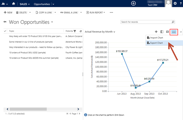
Modifying Chart XML in CRM 2013 — The Basics - Microsoft Dynamics CRM Community

How to Move Excel Pivot Table Labels Quick Tricks Use Menu Commands to Move Label. To move a pivot table label to a different position in the list, you can use commands in the right-click menu: Right-click on the label that you want to move. Click the Move command. Click one of the Move subcommands, such as Move [item name] Up. The existing labels shift down, and the moved label takes its new ...

33 Add Axis Label Excel 2016 - Label Design Ideas 2020

Excel Waterfall Chart: How to Create One That Doesn't Suck The first and last columns should be Total (start on the horizontal axis) and to set them as such, we have to double-click on each of them to open the Format Data Point task pane, and check the Set as total box. You can also right click the data point and select Set as Total from the list of menu options. Finally, we have our waterfall chart: 2.

34 Excel Graph Add Axis Label - Labels Database 2020

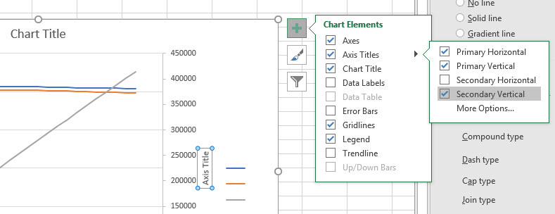
How to Add Axis Titles in a Microsoft Excel Chart Add Axis Titles to a Chart in Excel Select your chart and then head to the Chart Design tab that displays. Click the Add Chart Element drop-down arrow and move your cursor to Axis Titles. In the pop-out menu, select "Primary Horizontal," "Primary Vertical," or both.

Excel 2013 Recommended Charts, Secondary Axis, Scatter & PivotCharts

How to add secondary axis in Excel (2 easy ways) - ExcelDemy In this way, both the axis titles will be created. To add individual axis titles, go to Design tab (only available when a chart is selected) => Chart Layouts window => click on the Add Chart Element dropdown => hover your mouse over Axis Titles -> 4 options appear => Choose your preferred option

Add Secondary Value Axis to Charts in PowerPoint 2011 for Mac

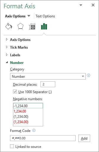
How to Change the Y Axis in Excel - Alphr Click on the axis that you want to customize. Open the "Format" tab and select "Format Selection." Go to the "Axis Options", click on "Number" and select "Number" from the dropdown selection under...

Bar-Line Chart with Secondary Axis or Two Panels - Peltier Tech Blog

Chart resets X axis every time I save. - Microsoft Community The problem does seem to be confined to one sheet. All of the charts are mixed type with x,y scatter with no lines (just points) and x,y scatter with smooth lines. I am using data labels with cell values on the points, but not the smooth lines. I am using Excel 2013 on Windows 7.

Changing Axis Labels in PowerPoint 2013 for Windows

Make Excel charts primary and secondary axis the same scale First create 2 new columns and call then Primary and Secondary Scale. In the first cell create a MIN function that looks at ALL the original data points and finds the smallest number. In the last cell do the same but this time a MAX to find the biggest number out of all the data points. In E8 and E34 just equals to the adjacent cells.

Changing Axis Labels In Excel 2016 For Mac

How to Change Axis Labels in Excel (3 Easy Methods) For changing the label of the Horizontal axis, follow the steps below: Firstly, right-click the category label and click Select Data > Click Edit from the Horizontal (Category) Axis Labels icon. Then, assign a new Axis label range and click OK. Now, press OK on the dialogue box. Finally, you will get your axis label changed.

Share :